Quickstart¶

This tutorial runs PeakATail end-to-end on a single BAM file. You will peak-call, cluster, run differential testing, and open the volcano figure — all in five steps.

Step 1 — Configure `example.yaml`¶

Copy the file from the repo root and edit the paths:

cp example.yaml my_run.yaml

The full content of example.yaml with explanations for every key:

# my_run.yaml
# Each dataset is one logical sample group. BAMs within a dataset share
# cell barcodes (same sequencing library — 10x, STARsolo, Alevin-fry, or
# any aligner emitting CB:Z / UB:Z tags). merge_strategy controls how
# multiple BAMs are combined before peak-calling (see Tutorial 3).
#
# merge_strategy options:
#   before  — merge all BAMs into one, then peak-call (more signal)
#   after   — peak-call each BAM separately, then merge PAS coordinates
#   none    — single BAM, no merging needed

datasets:
  - id: sample1
    merge_strategy: before
    bams:
      - /path/to/sample1_rep1.bam
      - /path/to/sample1_rep2.bam
  - id: sample2
    merge_strategy: none
    bams:
      - /path/to/sample2.bam

# GTF for gene annotation (Ensembl recommended)
gtf: /path/to/annotation.gtf

# Output directory (a timestamp suffix is added automatically)
output_dir: emaout

# Read geometry — match your sequencing protocol
seqlen: 150      # total read length
cb_len: 16       # cell barcode length: 10x v2/v3 = 16, Drop-seq = 12, etc.
barcode_tag: CB  # BAM tag holding the cell barcode

# Cell filtering
min_read: 1500   # minimum reads per cell barcode (low = too few PAS)
min_cells: 3     # minimum cells that must express a PAS to keep it
min_pas_per_cell: 50  # minimum PAS detected per cell (post-filter)
pas_gap: 100     # minimum bp gap between two PAS within one peak

# Optional: snap PAS to a reference atlas instead of calling de novo
# atlas: references/polyasite_2.0_GRCh38_sorted.bed
# atlas_distance: 50

Key field explanations pulled from ema/cli/config_schema.py::RunConfig:

Key	Type	Default	What it does
`datasets`	list	—	One entry per sample group. Required.
`gtf`	path	—	Ensembl GTF for UTR annotation. Required.
`seqlen`	int	—	Sequencing read length. Required.
`cb_len`	int	—	Cell barcode length in bp. Required.
`barcode_tag`	str	`CB`	BAM tag holding the cell barcode.
`min_read`	int	`1500`	Drop cells with fewer total reads.
`min_cells`	int	`3`	Drop PAS expressed in fewer than this many cells.
`min_pas_per_cell`	int	`50`	Drop cells with fewer PAS detected (maps to `filter_config.min_genes`).
`pas_gap`	int	`100`	Minimum bp between two PAS calls within the same genomic peak.
`atlas`	path	`None`	When set, PAS are snapped to the reference atlas instead of de-novo coordinates.
`atlas_distance`	int	`50`	Maximum snap distance in bp.

For a full list of parameters see ema run --help or the CLI reference.

Step 2 — Run the pipeline¶

uv run ema run --config my_run.yaml --threads 4

--threads 4 limits the parallel worker pool to four CPUs. Omit it to let PeakATail auto-detect your machine's core count.

The run will print a progress bar with one stage per pipeline phase (peak calling, CB filter, GTF annotation, PAS-gene assignment, annotated matrix, preprocessing, clustering). Typical wall time on a single-BAM human sample (~100M reads, 1000 cells) is 15-30 minutes.

Output lands in a timestamped directory:

peakatail_runs/emaout_<timestamp>/

Step 3 — Inspect what landed on disk¶

Each pipeline stage writes into its own numbered directory, with per-dataset data nested inside:

peakatail_runs/emaout_<timestamp>/
  01_peak_calling/sample1/
    pasbed.bed               # combined positive+negative PAS BED
    posbed.bed               # positive-strand PAS BED
    negbed.bed               # negative-strand PAS BED
    raw/                     # pre-filter snapshots: pos.bed, neg.bed, pas.bed, pos.mtx, neg.mtx, cb.tsv
  02_cb_filter/sample1/
    filtered_cb.tsv          # cell barcodes that passed min_read filter
  03_gtf_annotation/sample1/
    annotatedpas.bed         # pasbed.bed extended with a gene_id column
  04_pas_gene_assignment/sample1/
    pas_gene.tsv             # PAS-to-gene two-column mapping
  05_annotated_matrix/sample1/
    annotated_matrix.mtx     # PAS-by-cell count matrix (post gene annotation, pre filter)
    annotated_pas_ids.tsv    # PAS row index for the annotated matrix
    annotated_cells.tsv      # cell barcode column index for the annotated matrix
  06_preprocessing/sample1/
    preprocessed.h5ad        # AnnData after cell/PAS filtering, before clustering
  07_clustering/sample1/
    clusters.h5ad            # AnnData with leiden cluster labels — the main output

The clusters.h5ad is the primary artifact for all downstream analysis. Load it with:

import anndata as ad
adata = ad.read_h5ad("peakatail_runs/emaout_.../07_clustering/sample1/clusters.h5ad")
print(adata)
# AnnData object with n_obs x n_vars = <cells> x <PAS>
# obs: 'leiden', ...
# var: 'gene_id', ...

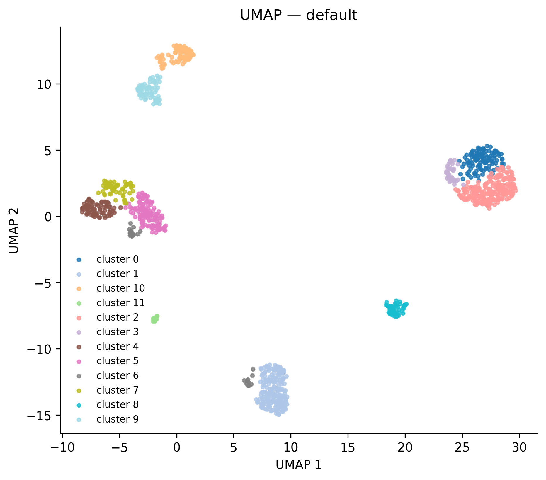UMAP — 12 clusters from the full_v8 run UMAP coloured by Leiden cluster. Each dot is a cell. Clusters are computed from 3'UTR usage patterns, not total expression, so cells that use similar polyadenylation sites cluster together regardless of overall RNA levels.

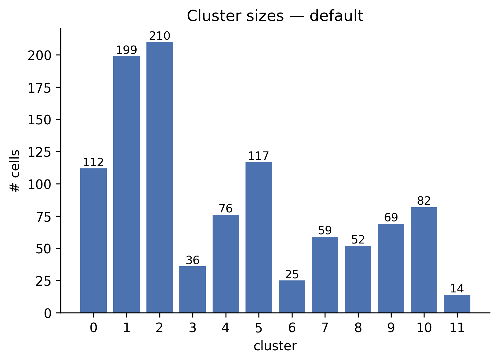Cluster sizes Bar chart of cells per cluster. The largest clusters (1, 2, 5) contain 117-210 cells; the smallest (11) has 14 cells.

Step 4 — Run differential testing¶

Point ema switch diff at the h5ad produced above:

uv run ema switch diff \
  --h5ad peakatail_runs/emaout_<timestamp>/07_clustering/sample1/clusters.h5ad \
  --pasbed peakatail_runs/emaout_<timestamp>/01_peak_calling/sample1/pasbed.bed \
  --strategy fisher \
  --fdr 0.05

Output lands inside the same run directory:

peakatail_runs/emaout_<timestamp>/switch_diff_<timestamp>/
  differential/
    fisher_0_vs_1.tsv
    fisher_0_vs_2.tsv
    ...   (one TSV per cluster pair)
  markers.tsv               # top-N marker PAS per cluster used to filter tests
  figures/
    volcano_0_vs_1.png
    volcano_0_vs_1.html
    ...
    figures_INDEX.md        # human-readable index of all figures
    figures_INDEX.json      # machine-readable manifest

Step 5 — Read the figures index¶

cat peakatail_runs/emaout_<timestamp>/switch_diff_<timestamp>/figures/figures_INDEX.md

This prints a table of every volcano figure with per-pair statistics. Example excerpt from the full_v8 run:

## `volcano` (66)

- **volcano_0_vs_4** (2 files) — cluster 0 vs 4 · n_tested=1433 · sig=935
- **volcano_3_vs_4** (2 files) — cluster 3 vs 4 · n_tested=1364 · sig=1058

Open volcano_0_vs_4.png to see which PAS drive the separation:

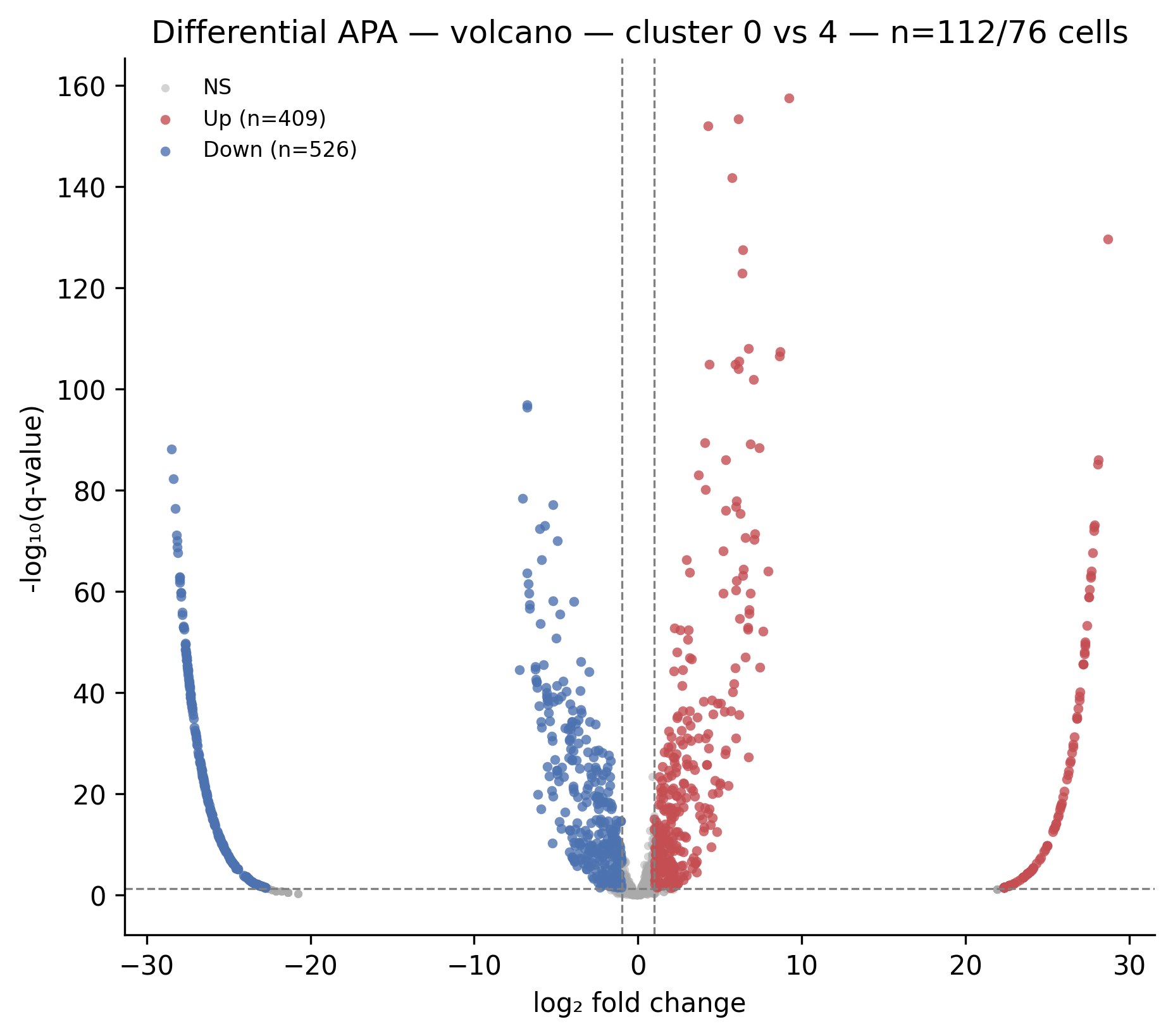Volcano: cluster 0 vs 4 Each dot is a PAS. Red = higher usage in cluster 4 (positive log2fc); blue = higher usage in cluster 0 (negative log2fc). The dashed horizontal line marks q = 0.05; dashed vertical lines mark |log2fc| = 1. The 0 vs 4 comparison shows 935 significant PAS out of 1433 tested.